How to X out a cell in Excel – a visual How-to

X out a cell in Excel

There are a couple ways to cross out a cell in Excel. My favorite way is shown first, but a more manual option is also shown right after the first. Both methods are outlined below.

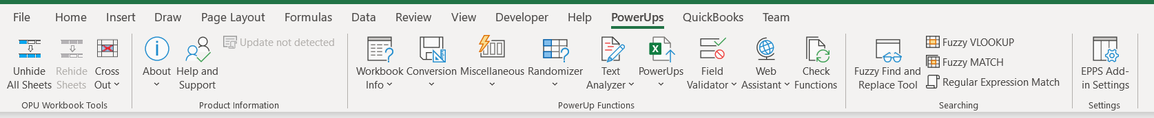
Method 1 (my favorite way to cross out a cell): Add a Small Tool – Make Excel Better

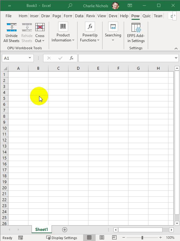
You can add a tool into Excel that will make it super easy to cross out cells. Or if a cell is crossed out, uncross it out. You can use the tool to set the line color, set the thickness of the line, and choose between a solid line or a dotted line for the “X”.

Or, you can right-click the highlighted cells and select Cross Out Cell(s) from the context menu.

You get these same menu options with the tool if you right-click in a cell. The menus fly out as you hover and make your selection.

The tool also also adds a feature to unhide all the hidden tabs. When you’re done looking at them you can re-hide them with a single click. As with the cross-out tool, you can right-click on a worksheet tab and you will have the unhide all and re-hide sheets available to you there too.

The added functionality makes it much quicker to cross out cells or to toggle hidden worksheet tabs on and off in Excel. There is no trial version of the basic OPU Workbook Tools for Excel add-in. However, there is a trial version of the Excel Powerups Premium Suite which includes the OPU Workbook Tools functionality. You can get that trial version from the Download link at the top of this page.

Method 2: Manually Format the Cell

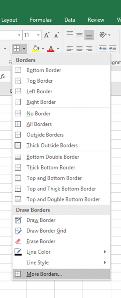
You can easily X out a cell in Excel by manually placing an X from corner to corner in a cell in Excel. Follow the steps below with the accompanying screen shots.

• The Format Cells dialog box appears. In the Format Cells dialog box, select the Border tab.

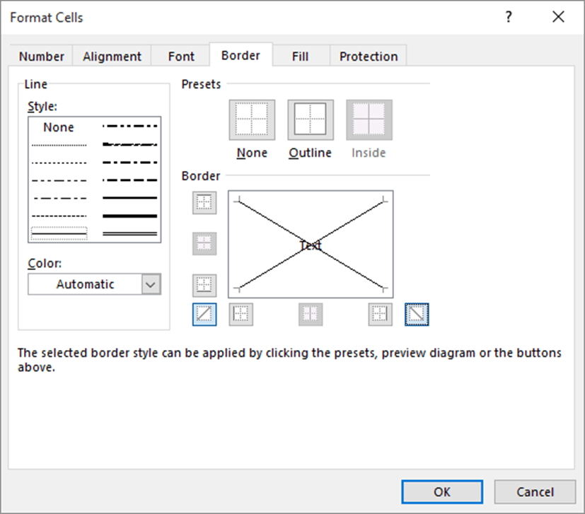
• Select both of the corner line buttons. There is one on either of the lower right and left corners of the big box in the center of the dialog box.

and

• Click OK.

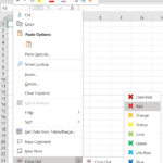
You can change the color of the X by changing the color of the lines used. Just change the selection in the Color drop down box from Automatic to the color you prefer.

If you want to uncross out the cell you can go back to the same Borders drop down list. On that list there is an option for No Borders. However, if you have any other borders (for example, you’re doing this in a table) selecting the No Border option will get rid of the table borders on any cells you’ve selected.

Alternatively, you can go back to the More Borders dialog box and unselect each of the diagonal corner line buttons.

So you can see if you have to do this more than once, it’s really not that feasible to do manually all the time. That’s why I use the OPU Workbook Tools for Excel tool mentioned above.

Also bundled into EPPS, you may already have OPU Workbook Tools for Excel

If you already have the Excel PowerUps Premium Suite, you already have the Cross Out tool. With a cell or range of cells selected you click the Cross Out Cell(s) button in the OPU Workbook Tools section of the PowerUps ribbon or in the context menu just as in the best method outlined above.

If you don’t see it in your current version, you can get the most recent version from https://officepowerups.com/update.