Two ways to add a drop down list in Excel
Sometimes you have a sheet that you need other people to fill in. And, you have a column or range of cells that need to have values from a specific set of values. You don’t want to have to deal with multiple variations of “yes”, for example. You might wind up with “Yes”, “1”, “True”, “Y”, “T”, and who knows what else. You need people to stick to the menu of choices to make your analytic life much easier. The solution: add a drop down list in Excel.
You’ve seen drop down pick lists in other people’s spreadsheets and want to do the same in yours. The process is pretty straightforward. I’ll describe a couple of common ways below. The option you pick would depend on the number and length of the items to pick from. A 60-second demonstration video is included at the end of this page as well.
Option 1, directly type the values in
If you want a simple pick list this might be the way to go for you. Think of having a list such as “Yes”, “No”, “Maybe” for example. To create a list with this option do the following.
- Select the cells you want to have the drop down list to pick values from.
- Select Data from the Excel ribbon.
- Select Data Validation from the Data Tools group.
- Select Data Validation…
- In the Validation criteria section, change the Allow drop-down box from Any Value to List.
- In the Source text box, enter the following:
- “Yes”, “No”, “Maybe”
- Click OK
At this point the cells you had selected will only allow one of the values you specified in the Source field (“Yes”, “No” or “Maybe” in this example).
Option 2, set values based on a range
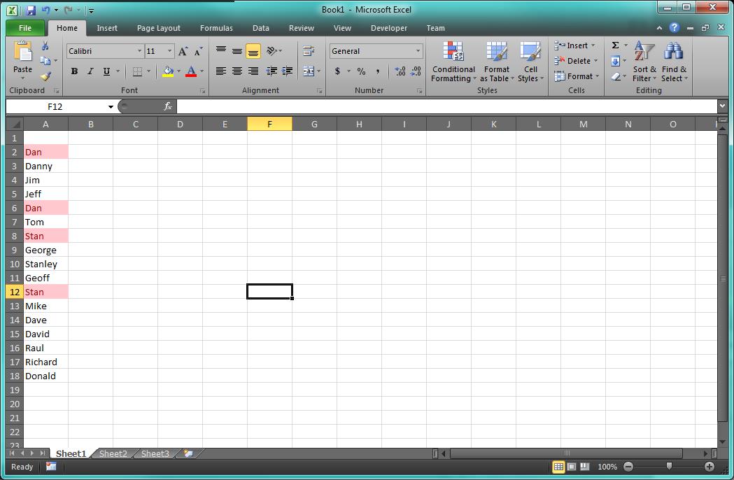
Option 1 above is a bit of a hassle if you have a longer list or if the values themselves are longer. In a case like this Excel makes it easy to have a list that you keep in a set of cells. These can be either on the same sheet or on another sheet. For example, imagine having the following values in cells A1 thru A10:
Amarillo
Banana
Citrus
Daffodil
Dandelion
Goldenrod
Hilighter
Post-it
Sunflower
Tulip
In order to easily make this list control the values in your pick list do this following.
- Select the cells you want to have the drop down list to pick values from.
- Select Data from the Excel ribbon.
- Select Data Validation from the Data Tools group.
- Select Data Validation…
- In the Validation criteria section, change the Allow drop-down box from Any Value to List.
- In the Source text box, enter the following:
-
=$A$1:$A$10
- Alternatively, you can simply highlight the block of cells and the cell range above will automatically be put in the Source box.
-
- Click OK
At this point, just as in Option 1 above, the cells you had selected will only allow one of the values you specified in the Source field (Some form of yellow in this example).
Demo
Here’s a short video example to see how easy it can be to add a drop down list to Excel.
There you go.


Thank you, simply explained and worked first time 🙂
Excellent walk through.
Created it just like the excellent walk through; however, when I select an item from the drop down list, the next cell has 2 of them and deletes the 1st choice.
Hi Joanna, I’ve tried to come up with a scenario that does what you’ve described but I can’t duplicate what you’ve experienced.
My selection list has coloured cells (different background and ink colours for each cell in the list) . When I select the option form the dropdown menu though, the text and the cell are just black and white and not coloured.. Why ?
That’s just the way Excel does it. Everything in the list is the same. If you change the font in your source list you’ll notice the font isn’t passed thru to the drop down list either.
If you want to make an item stand out you can indent it (pad it with spaces) and the indentation will show up in the list.
HTH