
I’ve used VLOOKUP for many many years. It’s a straightforward enough concept: scan down a column for a match in a cell, then look over to the right in that row for the value we want to retrieve. And, all of this is wrapped into a single function call: VLOOKUP.
But you may have found VLOOKUP has a particular limitation. It can only look to the right of the cell you’ve matched. If you’ve been able to plan ahead and lay out your data so that the column you’re scanning is to the left of the range of information you’re looking for, you’re in luck I suppose.
But if you’re like me and your data is provided to you from another source or you don’t always envision every use of the data beforehand you may wind up needing to search a column in the middle of your range. And further, the data you need to retrieve is to the left of your search column. VLOOKUP won’t help: it only looks to the right.
VLOOKUP to the left, more or less
Fortunately, there is a very powerful duo of functions in Excel that effectively let you do a VLOOKUP to the right or to the left.
Meet INDEX-MATCH
I’d like you to meet the INDEX and MATCH functions. These two functions are very often used together and they give you the bidirectional lookup you need. You’ll no longer be limited to looking to the right.
Here are the main steps involved.
1. You’ll use the MATCH function to find the row number of the cell that contains the value to find. By itself, you’d write the function similar to the following:
=MATCH(lookupvalue, lookuprange)
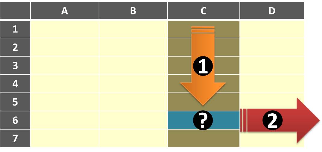
“lookupvalue” is just the value that you’re trying to find in the column — arrow #1 above.
“lookuprange” is just the table column reference or the range of cells to search within — the brown cells in the image above.
Look at the image above. If you were to use MATCH and find the your “lookupvalue” in the cell highlighted in blue above, the MATCH function would return a value of 6. This is the row index of the match.
Note: if you want to do an exact match just return a third parameter of FALSE like you would in VLOOKUP (=MATCH(lookupvalue, lookuprange, false)).
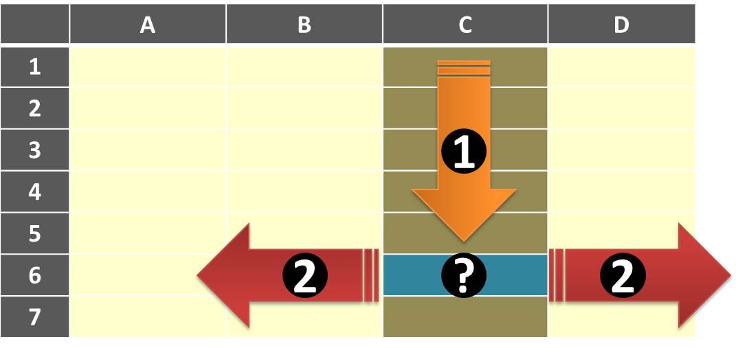
2. Next you’ll use the INDEX function to look in another column that has the data you’re trying to retrieve. This column can be either to the left or the right of your lookuprange. You won’t actually specify a column number as you would have in VLOOKUP. Instead, you can pick any column. By itself, you’d write the INDEX function similar to the following:
=INDEX(columnrange, rownumber)
Look at the image above again. Once you have the row number from the MATCH function you can look to either side for the data to return.
3. The combined usage of these two functions is really what you’ll be doing. Since the MATCH function returns the row number of the match you will insert (or nest) the MATCH function as one of the parameters of the INDEX function. It looks like this:
=INDEX(columnrange, MATCH(lookupvalue, lookuprange))
Don’t let the more complicated look of the two functions turn you off. Its a straightforward change in the way you match and cross-reference values to use and you get all the power of the combined functions.
Do you need to do a fuzzy match? See Fuzzy VLOOKUP in Excel.
There you go.