Ok, you have a set of values in a column or a row and you want to find out if any of those values exist in another list (which could be in either a row or a column elsewhere).
You can do that in Excel by using the MATCH function to test for a specific value in another range. We’ll look at that below.
Worksheet setup
First, let’s set up a worksheet example. You can replace with any values you like of course.
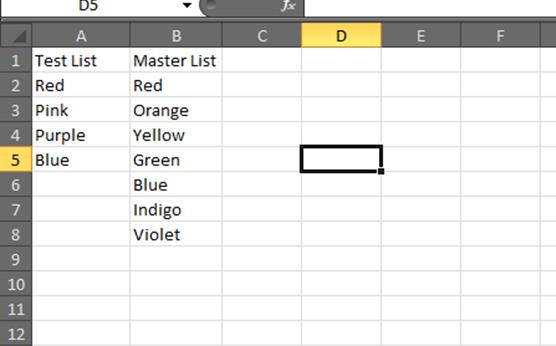
Here’s a list we want to find duplicates from. Think of this as your ‘Test’ or source list.
Red, Pink, Purple, Blue
Here’s a list that we want to look into. Think of this as our ‘Master’ list.
Red, Orange, Yellow, Green, Blue, Indigo, Violet
Here’s the formula to use for this particular example. In your case, you’d change the range to match the row or column that contained your Master list of data. The size of your Master list doesn’t need to match the size of your Test list. It also doesn’t matter if your range is in a column or in a row – it’s just a series of cells that contain your master list.
=IFERROR(MATCH(A2,$B$2:$B$8,0),0)Note that the dollar signs (“$”) in the cell references are important. They make the references “absolute” so they don’t shift as you apply the formula to other cells. If you want to read a bit more about an absolute reference you can take a look at another post of mine about absolute versus relative references.
We can put that formula in a number of places. It just depends on what you want or need to do with the result. Let’s take a look at a couple examples.
Example 1
First, for the sake of illustration let’s just put the formula into C2 and then fill down alongside the values in the Master list. You can see a bunch of numbers.
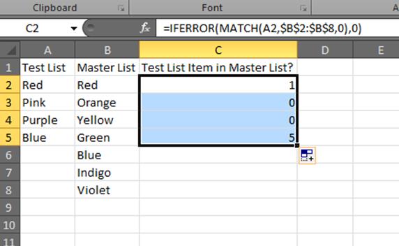
Basically, “0” means “not found” and “not zero” means “found”. We’ll talk in more detail below on this as we break down the formula.
Example 2
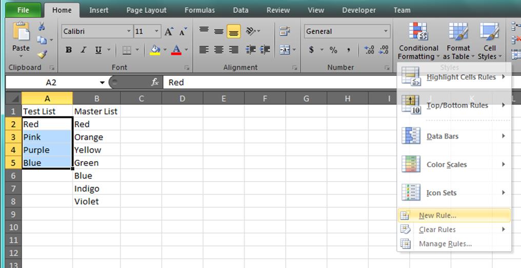
Here’s another illustration using Conditional Formatting to highlight the existence, presence, or duplication of the Test value in the Master list. Start by selecting all of the cells in your Test list and perform the following steps.
- Click Conditional Formatting from the Styles group.
- Select New Rule from the menu.

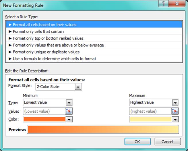
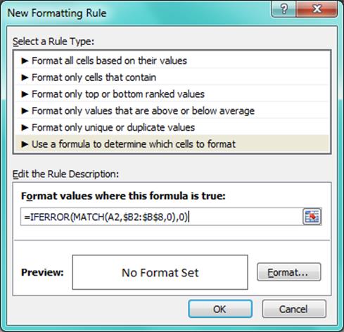
- Select Use a formula to determine which cells to format from the Select a Rule Type box.
- Enter the formula from above into the Format values where this formula is true box.
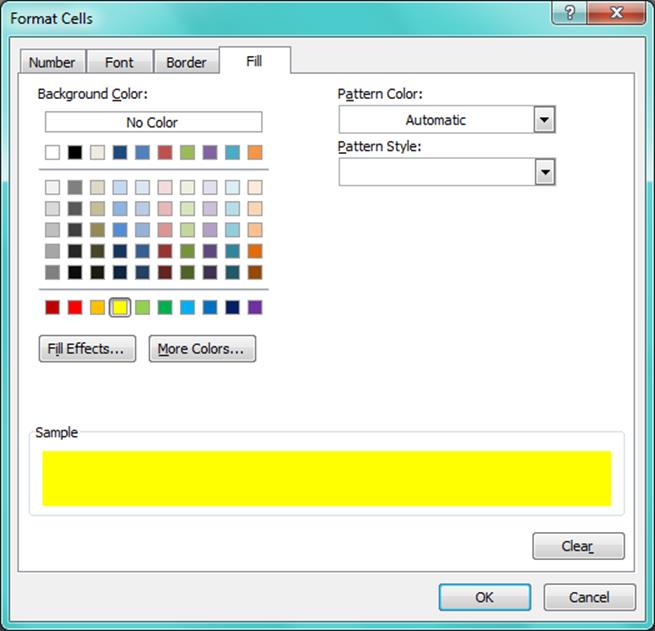
- Click the Format button, then click the Fill tab.
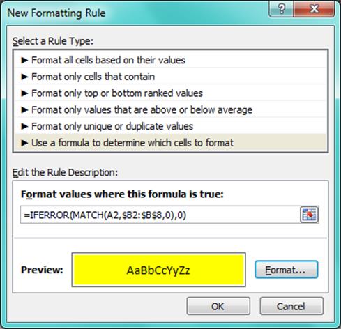
- Pick a Background Color. Let’s pick bright yellow. Now, you should be looking at an image like the one above.
- Click OK. You should see this:
- Click OK again. You should see this:
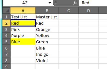
See? Now you’ve detected each duplicate value and can easily see them in the list.
Ok, let’s break down that formula
Meet MATCH
The MATCH function is a built-in function in Excel. It does just what its name implies: it matches a value against a set of values. And, based on that it will give back a number to your spreadsheet. If no match was found, a “#N/A” error is returned. Any number represents where in the list the match occurred (you can use that to your advantage in other scenarios). For our needs here, a number value being returned just means “match found”.
So “A2” is the first value in your Test list. This value will automatically adjust to “A3, A4..” as you fill down.
The $B$2:$B$8 just defines the range of your Master list which is between cells B2 and B8. You can change this to any set of rows or columns that work with your data. Rows would just have the letters changing instead of the numbers (such as $A$2:$F$2).
Finally, the “0” in the third parameter slot is just saying find an Exact Match.
Meet IFERROR
The MATCH function is used inside or nested within the IFERROR function. The only thing that the IFERROR function does is return one value if it doesn’t detect an error, and another value if it does detect an error. So in this case, IFERROR will return the number from the MATCH function if a match was found and will return a “0” (the second parameter of the IFERROR function) if an error is found.
So in the end, the combination of these functions will return a 0 or a number. We used this fact in the Conditional Formatting example above because a “0” means “False” and non-zero means “True”. This is how the Format values, where this formula is true, is assessed when Excel decides whether to apply the formatting.
There you go. I hope this was helpful.