Excel has a number of functions that will look up a value based on finding a corresponding value in a range, row, or column.
Meet LOOKUP
The Excel LOOKUP function matches a value you’re looking for in a row or column and then returns the value from another matching row or column. I tried to create a visual to help.
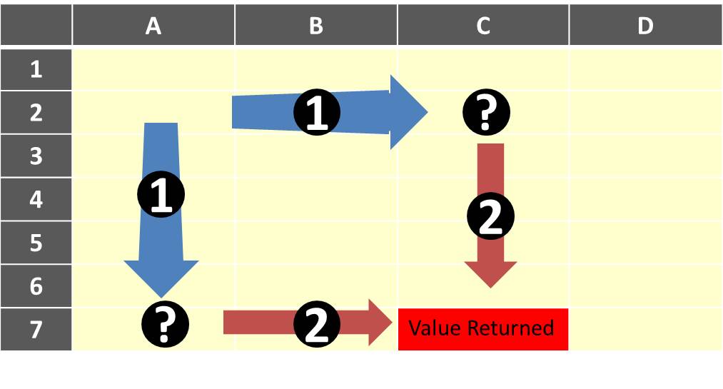
Part 1 in the image is LOOKUP finding the value you’re looking for (represented by the “?”).
Part 2 is LOOKUP finding the corresponding value in the column or row you specify. So the value returned (shown in red above) is the value you were looking for based on the initial value you were matching.
Note that in the picture above, both looking up by row and by column are depicted. Just look at the 1 & 2’s by rows, or by columns.Here’s what the above may look like as a function. Imagine you want to find the name of a customer based on their phone number.
=LOOKUP("555-1212", A2:A7, C2:C7)
This would match the phone number in the range of cells defined above in column A, and then find the value from the corresponding cell in the range between C2 and C7.
If your lookup data isn’t sorted in ascending order the LOOKUP function won’t work as expected. This is an unfortunate limitation of Excel.
Alternative form of LOOKUP
This might seem a bit confusing. If so, this additional information probably won’t help. LOOKUP has another form (called the “array” form versus the “vector” form above). In the array form, you only need to specify the value to look for and the upper-left cell and the lower-right cell of the range or “array”.
The same example from above may be written such as the following.
=LOOKUP("555-1212", A2:C7)
Imagine a box whose upper left and lower right corner coordinates were A2 and C7.
There you go.