excel Archives - Page 2 of 8

04Nov 2015 by Charlie Nichols No Comments

Concatenate a range of cells in Excel – Easily

200 level, Excel

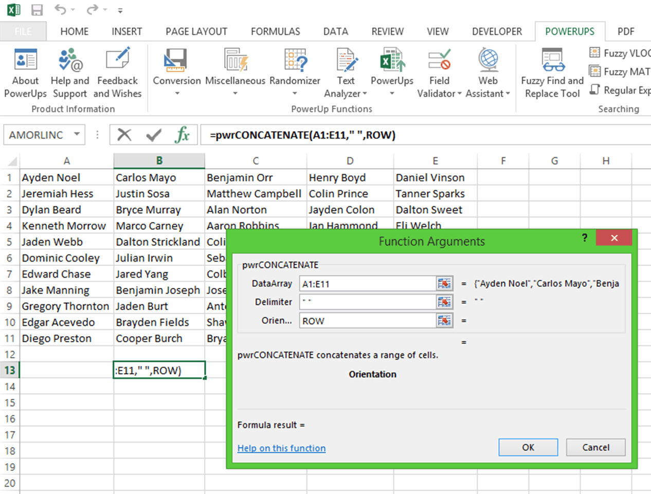
[wp_ad_camp_1] Concatenate a Range of Cells in Excel Concatenate a range of cells in Excel without having to individually select every cell that you want to concatenate. The pwrCONCATENATE function (part of the Text Analyzer Assistant in the Excel PowerUps Premium Suite) lets you select a range of cells to concatenate. Additionally, you can add a delimiter between the concatenated cells if you wish. Also, you have control over whether to concatenate rows first or columns first. You can have empty cells in the range. They'll just be skipped. For example, you can use the following formula. =pwrCONCATENATE(E3:G30, " ", "COL") This will concatenate the range of cells between cells E3 and G30. Each cell will have a space (" ") character inserted between and the concatenation will go in the…

27Oct 2015 by Charlie Nichols 1 Comment

How to X out a cell in Excel – a visual How-to

100 level, Excel

[wp_ad_camp_1] [wp_ad_camp_4] X out a cell in Excel There are a couple ways to cross out a cell in Excel. My favorite way is shown first, but a more manual option is also shown right after the first. Both methods are outlined below. Method 1 (my favorite way to cross out a cell): Add a Small Tool - Make Excel Better Easily cross out cells with a click You can add a tool into Excel that will make it super easy to cross out cells. Or if a cell is crossed out, uncross it out. You can use the tool to set the line color, set the thickness of the line, and choose between a solid line or a dotted line for the "X". Or, you can right-click the highlighted…

05Oct 2015 by Charlie Nichols No Comments

How to fix a VLOOKUP error in Excel

200 level, Excel

[wp_ad_camp_1] [wp_ad_camp_4] VLOOKUP error in Excel Ever have this happen? You write your VLOOKUP formula and have one of the following values returned: #VALUE! #NAME? #N/A #REF! Other UNEXPECTED result! Below you’ll find some common pitfalls that cause each of the errors above. VLOOKUP function syntax First, here’s a recap of the usage syntax for the VLOOKUP function in Excel. I’ll be referring to the parts in the explanations below. VLOOKUP(lookup_value, table_array, column_index_number, [range_lookup]) For more detail on the arguments, see the function's documentation page. VLOOKUP errors in Excel #VALUE! error causes in VLOOKUP column_index_number is less than 1 In an effort to retrieve a value that is to the left of the lookup column, you may be tempted to put in a value less than one. However, VLOOKUP only finds…

27Sep 2015 by Charlie Nichols No Comments

Excel Financial Functions tutorial

200 level, Excel

[wp_ad_camp_1] [wp_ad_camp_4] Excel as a Financial Tool Excel provides a number of functions to make calculating financial data very easy. You can find a great deal of examples and documentation on each of the functions. For this tutorial, we will use five commonly used Excel financial functions and use them together to answer some common questions. Excel Financial Functions The Excel financial functions that we will use in this tutorial are the following. PMT RATE NPER PV FV Each of these can be use to answer a likely question in the scenario for our tutorial. In this example, we'll consider the purchase of a used car and answer the following questions. What is my payment going to be? If I pay more than the minimum payment, how much earlier would…

21Sep 2015 by Charlie Nichols No Comments

Regular Expressions in Excel – Test Tool

200 level, Excel

[wp_ad_camp_1] [wp_ad_camp_4] Regular expressions in Excel Regular expressions in Excel are made easy with the pwrREGEXMATCH function. As a demonstration of the function, the example file pictured below is set up to evaluate a regular expression entered in cell D2 against text entered in cell D4. The result is contained in cell D8. The formula used in Excel (cell D8) is the following: =pwrREGEXMATCH(D4, D2) That's it. Download the example worksheet (link below) or just create one on your own. Using this, you can easily try out different regular expressions against some target text to massage into the perfect regex for your need. [caption id="attachment_3430" align="aligncenter" width="908"] Sample Excel template demonstrating use of regular expressions in Excel thru the pwrREGEXMATCH add-in function[/caption] Download the sample workbook here.

24Jun 2015 by Charlie Nichols No Comments

How to drag and drop columns in Excel

100 level, Excel

[wp_ad_camp_1] [wp_ad_camp_4] This is a quick little tip that makes it really easy to move columns of data around in Excel. It's basically a drag and drop operation - basically. In the example below, we'll just move the data in column C over to column B. When done, the column headings will be in order: First Column; Second Column; Third Column. [caption id="attachment_3350" align="alignnone" width="588"] Sample worksheet[/caption] First, select the entire column. To select a column, click the column heading (one of the letters or double-letters). Don't select a cell and try and highlight everything - just click the column heading. In this example, click the "C" so that we can move column C. [caption id="attachment_3351" align="alignnone" width="586"] Select the column to move[/caption] Next, hover your cursor over one of…

07May 2015 by Charlie Nichols No Comments

How to calculate compound interest in Excel

200 level, Excel

[wp_ad_camp_1] [wp_ad_camp_4] Compound Interest Compound interest is interest added to the principal and interest earned in previous periods. This addition of interest to the principal is called compounding. Just below you can see how to calculate compound interest in Excel. The formula for calculating compound interest is =PV*(1+R)^N How to calculate compound interest in Excel The formula above is entered in Excel as =PV*(1+R)^N In the formula, PV is the present value. R is the interest rate. And N is the number of periods (such as annually) that you want to compound. Example Suppose you have $1000 to start with. Your present value (PV) would be 1000. If you expect to earn 7% annual interest, your rate (R) would be .07. To see how much you would have after 10…

03Feb 2015 by Charlie Nichols No Comments

How to compare two strings in Excel

200 level, Excel

[wp_ad_camp_1] [wp_ad_camp_4] How to Compare Two Strings in Excel for Similarity Excel comes loaded with several useful text or string comparison functions. Out of the box, Excel provides a function named EXACT that will return whether two strings are exact matches. That's great, unless you actually need to find strings that are really close or very similar. The good news is when you want to compare two strings in Excel you aren't limited to exact matches only. Using a function such as pwrSIMILARITY you can compare two strings and get a rating back (a percentage) that indicates the degree of similarity between the two strings. You actually have a great deal more flexibility with pwrSIMILARITY. For example, the EXACT function is case sensitive so comparing "Abc" and "abc" would return…

22Jan 2015 by Charlie Nichols No Comments

How to Generate Random Text in Excel

200 level, Excel

[wp_ad_camp_1] [wp_ad_camp_4] A Little About Lorem Ipsum "Lorem Ipsum" text is commonly used in the printing or design industry as dummy text used as a placeholder for "real" text. The Lorem Ipsum text is originally from Latin literature that is over 2,000 years old. It is not Latin-looking gibberish as often believed. Generate Random Text in Excel You can use the pwrRANDOMTEXT function in Excel to generate random text. The random text generated will be based on the Lorem Ipsum text commonly used as filler. This function is available as part of the Random Data Assistant contained in the Excel PowerUps Premium Suite add-in for Excel. In order to use this function you simply use it in your worksheet as you would any other function. Examples If you want to…

08Dec 2014 by Charlie Nichols No Comments

How to Hide Gridlines in Excel

100 level, Excel

[wp_ad_camp_1] [wp_ad_camp_4] I've got this question several times. How do you hide the gridlines in Excel? It's a really quick task as you can see below. For each of Excel 2013, Excel 2010, and Excel 2007 you can click the View tab in the Ribbon. In the Show group, uncheck the Gridlines checkbox. Now you know how to hide gridlines in Excel. To show gridlines in Excel, just check the Gridlines box. There you go.