Excel as a Financial Tool

Excel provides a number of functions to make calculating financial data very easy. You can find a great deal of examples and documentation on each of the functions. For this tutorial, we will use five commonly used Excel financial functions and use them together to answer some common questions.

Excel Financial Functions

The Excel financial functions that we will use in this tutorial are the following.

• PMT
• RATE
• NPER
• PV
• FV

Each of these can be use to answer a likely question in the scenario for our tutorial. In this example, we’ll consider the purchase of a used car and answer the following questions.

• What is my payment going to be?
• If I pay more than the minimum payment, how much earlier would I pay off my car?
• How much can I borrow?
• How much will I owe later?
• What interest rate am I being charged?

Excel Financial Functions Tutorial

In order to illustrate the five selected Excel financial functions meaning and usage we’ll consider a series of questions you may have when purchasing a used car.

What is my payment going to be?

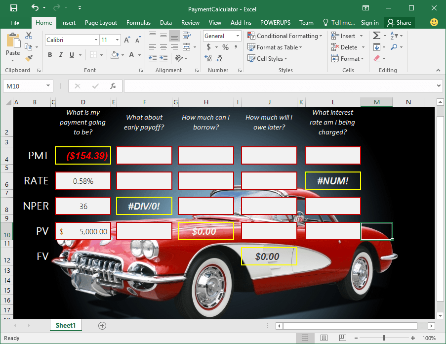
For the sake of illustration, let’s assuming you’ll be able to purchase the car without a down payment. And in this example we’ll say you’re going to borrow $5,000 to purchase the car. Also, we’ll assume an annual 7% interest rate for a 36-month loan.

To answer this question, you supply the information available to the PMT (payment) function in Excel. PMT is one of the Excel financial functions and takes up to five parameters. The last two are optional so we’ll use the first three.

The first parameter is the rate. In this example, our annual rate was 7%. To get our monthly rate we’ll just divide the 7% by the 12 months of the year. So we’ll use 0.005833 (0.07/12) as the rate.

The next parameter is the number of periods or payments. Here, it will be 36 for the 3-year loan.

The last parameter is the present value (PV) of the loan. For your hypothetical car, this will be $5,000.

The function we would type into Excel would be the following.

=PMT(0.005833, 36, 5000)

The value returned is -154.39. It’s a negative value (you pay that money out versus receiving it).

If I pay more than the minimum payment, how much earlier would I pay off my car?

In the example above, you figured out you would have a $154.39 monthly payment to pay off your $5,000 in 36 payments. But, what if you paid more than the minimum payment? How many months would be saved if you paid a bit more. Say, $175 monthly?

To figure this out you will use the NPER (number of periods) function in Excel. NPER is another one of the Excel financial functions and also takes 5 parameters. The last two are optional and we will only use the first three in this example.

The first parameter is the rate. This will be the same 0.58% (0.005833).

The second parameter is the payment amount you’d be paying. This will be $175. Remember this needs to be entered as a negative number.

The third parameter is present value, or in this case the amount of the loan. In this example, this is $5,000.

The function you type into Excel would be the following.

=NPER(0.005833,-175,5000)

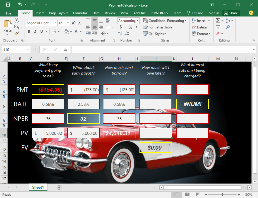
Rounding up to the nearest whole number, Excel returns 32 in this case. So by paying $175 each month instead of the minimum $154.39, you would have your car paid off four months earlier.

How much can I borrow?

Let’s say you know you’ll need to borrow in order to purchase a car. However, you’re not sure how much you can actually afford to borrow. Let’s say you’ve figured out you can pay $125 each month. And, the bank is offering a 7% loan for 36 months.

In order to figure out how much you could borrow in this case you would use the PV (present value) function in Excel. PV is another one of the Excel financial functions and takes up to five parameters. The last three are optional and we will only use the first three in this example.

The first parameter is the rate. The rate (monthly) will be the same 0.005833 (0.07/12) from above.

The second parameter is the number of periods. The number of periods will be 36 (3 years, 12 months/year).

The third parameter is the amount of the payment. In this example, you’d decided to limit the payment to $125. And remember the payment needs to be entered as a negative number.

The function you would type into Excel would be the following.

=PV(0.005833, 36, -125)

Excel will return $4,048.31. This would be the maximum amount you could borrow for a 3-year loan at 7% interest if you were to limit the payment to $125.

How much will I owe later?

Now, let’s say you have that $5,000 loan, for 36 months, at 7% annually, with a monthly payment of $154.39. And let’s say you actually only pay $150 monthly instead of the full $154.39. Ok, this is totally hypothetical because nobody would pay less than the required amounts every month. But for the sake of illustration let’s say you decided to and were able to pay just $150 monthly.

In order to see how much you would owe at the end of the 36-month term you would use the FV (future value) function in Excel. FV is one of the Excel financial functions and takes up to five parameters. For this example, we’ll use only the first four.

The first parameter is the rate. In this example the rate was 7% annually. We’ve figured out above that this works out to 0.58% (0.005833) monthly.

The second parameter is the number of periods. The number of periods will again be 36.

The third parameter is the amount of the payment. The payment we’ll say you’ve decided to pay instead will be $150. Again, remember this must be entered as a negative number.

And the fourth parameter is the present value, or the amount of the loan. In this example, this is $5,000.

The function you would enter into Excel would be the following.

=FV(0.005833, 36, -150, 5000)

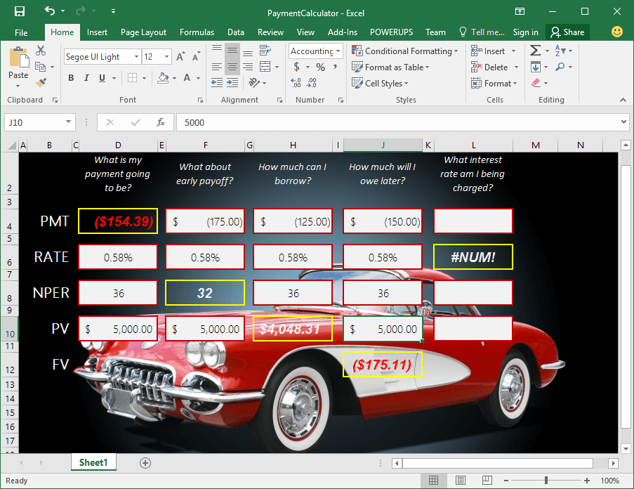
Excel will return $175.11. That would be (in theory) the amount that was unpaid on your loan at the end of the term.

What is the interest rate I’m being charged?

Have you ever had the experience of buying a car, and the sales person only talks about a monthly payment? It come across like they’re just working with your budget. You know, they’re just helping you out.

Let’s take a closer look at what’s going on.

For starters, let’s go back to the $125 monthly payment amount from the example above. And let’s stick with the 36-month payment period. For the amount borrowed, let’s say it was an even $4,000.

You can calculate the interest rate you are paying by using the RATE function in Excel. RATE is the last of the Excel financial functions we are learning about here. It takes up to six parameters. The last three are optional and we’ll only use the first three for this example.

The first parameter is the number of periods. This will be 36.

The second parameter is the amount of the payment. This will be $125. Which will be entered as -125.

The third parameter is the present value or the amount of the loan. This will be $4,000.

The function you enter into Excel would be the following.

=RATE(36,-125,4000)

Excel returns 0.65%. This the monthly rate. To get the annual we’ll just multiply by 12. So the following formula gives the annual rate.

=RATE(36,-125,4000)*12

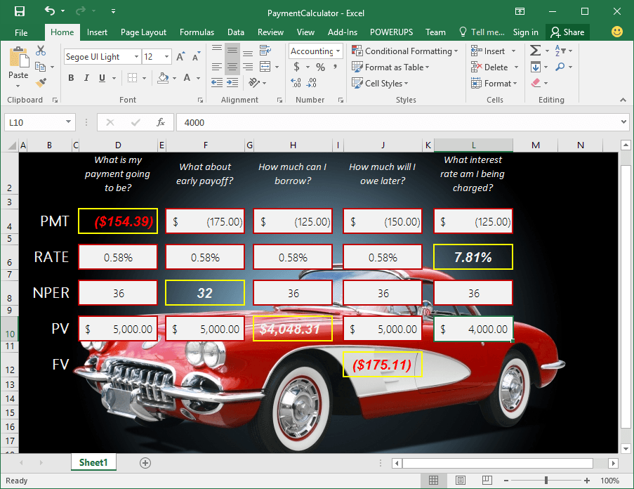
You can see that the rate you’d be paying to get a 36-month, $4,000 loan with a $125 monthly payment is 7.81%. You would be paying much higher rate compared to the 7% examples we’ve used up to now.

Download the Sample Workbook

If you wish, the workbook pictured above has been made available in the resource library. You can download the sample file with this PaymentCalculator link.

Additional acknowledgements

Yes, the actual cost of the loan will likely be higher (fees and such).

Yes, the actual cost of owning a car goes way beyond making loan payments. This is a conversation I repeatedly have with each of my kids.

Yes, these scenarios are simplified for the purpose of illustration. Many more financing variants exist.

These examples help illustrate the usage of the PMT, NPER, PV, FV, and RATE functions in Excel.

There you go.