In the example below, an Excel moving average formula is set up. It averages the values from a trailing number of days. For the initial set of days, it averages the available days and becomes a trailing or moving average after the desired number of days have passed. You can also modify this to just show a 0 for the days leading up to the first set to be averaged.
Excel moving average formula
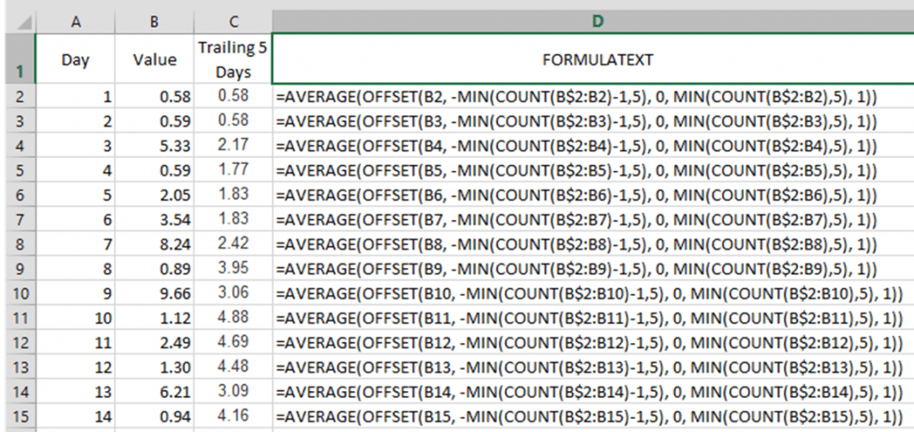
Here’s the formula I used, for those that just want to grab and go. It’s set up to calculate the 5-day moving average of the Value column. The figure below shows the worksheet used in this example.
[codeblocks name=”Moving average formula”]Put this formula in the first cell you want to begin the moving average calculation. Then, grab the fill-handle and drag the formula down as far as you need. The relative references will automatically adjust.
The rest of this article provides more of an explanation of how the formula is set up and why.
Breaking down the Excel moving average formula
Functions to use
We’ll use the following built-in Excel functions for this formula.
AVERAGE – this will do just what we want: get the average of a set of values.
OFFSET – we’ll use this to define the range we want to include in the values to average.
MIN – this will be used primarily to handle the case in the beginning where we don’t yet have the full number of days to average.
COUNT – this will be used, along with the MIN() function, to identify whether we have the number of desired data points for the number of days.
Calculation steps for the Excel moving average formula
COUNT(B$2:B2)
=AVERAGE(OFFSET(B2, -MIN(COUNT(B$2:B2)-1,5), 0, MIN(COUNT(B$2:B2),5), 1))
This part of the formula uses a combination of relative and fixed references. As you fill the formula down to more cells in Excel, the relative references will automatically adjust. So in the next row, B$2:B2 will automatically become B$2:B3. And so on.
The COUNT function will return the number of items in the range. At first, B$2:B2 is a range of one. As you fill down, the size of the range will automatically grow, as will the COUNT value returned.
-MIN(…-1,5)
=AVERAGE(OFFSET(B2, -MIN(COUNT(B$2:B2)-1,5), 0, MIN(COUNT(B$2:B2),5), 1))
The MIN function will return the lowest value of the set. Here, there are two values being compared. The first is the size of the range from the previous step, minus one. One is subtracted here because the initial offset we will need is zero. This parameter of the OFFSET function is the rows offset.
We also take the negative of the MIN value. As we copy this formula down in Excel, the negative value will make the range look “up”.
MIN(…,5)
=AVERAGE(OFFSET(B2, -MIN(COUNT(B$2:B2)-1,5), 0, MIN(COUNT(B$2:B2),5), 1))
This part of the OFFSET function parameter set is the height of the range. So, the MIN function will return the smaller of the number of available data points or the value of 5. We use 5 here because we want the 5 day moving average.
OFFSET(B2, …, 0, …, 1)
=AVERAGE(OFFSET(B2, -MIN(COUNT(B$2:B2)-1,5), 0, MIN(COUNT(B$2:B2),5), 1))
The remaining parameters of the OFFSET function are the initial reference (“B2”), the column offset (“0”), and the width of the range (“1”).
We use B2 as the beginning reference. This is a relative reference (no $ signs) so as this formula is filled down, the row number will automatically increase.
We’ll use the value of 0 for the column offset. Basically, we aren’t offsetting by the column at all in this example.
Finally, the width of the range we’re working with is one (just the single column) so we use the value of “1” for the final parameter.
AVERAGE(…)
=AVERAGE(OFFSET(B2, -MIN(COUNT(B$2:B2)-1,5), 0, MIN(COUNT(B$2:B2),5), 1))
Finally, the AVERAGE function gets passed a range of cells. With all of the above parameters used in the OFFSET function, the range returned to the AVERAGE function will be up to 5 consecutive cells with the range shifting down as the formula fills down.
There you go.